19 Improving performance

19.1 Checking for existing solutions

Q1: What are faster alternatives to lm? Which are specifically designed to work with larger datasets?

A: The CRAN task view for high-performance computing provides many recommendations. For this question, we are most interested in the section on “Large memory and out-of-memory data.” We could for example give biglm::biglm(),²⁷ speedglm::speedlm()²⁸ or RcppEigen::fastLm()²⁹ a try.

For small datasets, we observe only minor performance gains (or even a small cost):

penguins <- palmerpenguins::penguins

bench::mark(
  "lm" = lm(
    body_mass_g ~ bill_length_mm + species, data = penguins
  ) %>% coef(),
  "biglm" = biglm::biglm(
    body_mass_g ~ bill_length_mm + species, data = penguins
  ) %>% coef(),
  "speedglm" = speedglm::speedlm(
    body_mass_g ~ bill_length_mm + species, data = penguins
  ) %>% coef(),
  "fastLm" = RcppEigen::fastLm(
    body_mass_g ~ bill_length_mm + species, data = penguins
  ) %>% coef()
)
#> # A tibble: 4 x 6
#>   expression      min   median `itr/sec` mem_alloc `gc/sec`
#>   <bch:expr> <bch:tm> <bch:tm>     <dbl> <bch:byt>    <dbl>
#> 1 lm            1.3ms    1.5ms      653.  908.45KB     6.28
#> 2 biglm      963.69µs   1.07ms      911.    5.43MB     8.37
#> 3 speedglm     1.69ms   1.76ms      516.   62.34MB     6.24
#> 4 fastLm     988.31µs   1.04ms      935.    3.42MB     6.21

For larger datasets the selection of the appropriate method is of greater relevance:

eps <- rnorm(100000)
x1 <- rnorm(100000, 5, 3)
x2 <- rep(c("a", "b"), 50000)
y <- 7 * x1 + (x2 == "a") + eps
td <- data.frame(y = y, x1 = x1, x2 = x2, eps = eps)

bench::mark(
  "lm" = lm(y ~ x1 + x2, data = td) %>% coef(),
  "biglm" = biglm::biglm(y ~ x1 + x2, data = td) %>% coef(),
  "speedglm" = speedglm::speedlm(y ~ x1 + x2, data = td) %>% coef(),
  "fastLm" = RcppEigen::fastLm(y ~ x1 + x2, data = td) %>% coef()
)
#> # A tibble: 4 x 6
#>   expression      min   median `itr/sec` mem_alloc `gc/sec`
#>   <bch:expr> <bch:tm> <bch:tm>     <dbl> <bch:byt>    <dbl>
#> 1 lm           57.1ms   57.1ms      17.5      27MB    140. 
#> 2 biglm        54.7ms   54.7ms      18.3    22.2MB    128. 
#> 3 speedglm     36.7ms   41.2ms      23.4    22.9MB     41.0
#> 4 fastLm       66.1ms   66.1ms      15.1    30.2MB     75.6

For further speed improvements, you could install a linear algebra library optimised for your system (see ?speedglm::speedlm).

The functions of class ‘speedlm’ may speed up the fitting of LMs to large data sets. High performances can be obtained especially if R is linked against an optimized BLAS, such as ATLAS.

Tip: In case your dataset is stored in a database, you might want to check out the {modeldb} package³⁰ which executes the linear model code in the corresponding database backend.

Q2: What package implements a version of match() that’s faster for repeated lookups? How much faster is it?

A: A web search points us to the fastmatch package.³¹ We compare it to base::match() and observe an impressive performance gain.

table <- 1:100000
x <- sample(table, 10000, replace = TRUE)

bench::mark(
  match = match(x, table),
  fastmatch = fastmatch::fmatch(x, table)
) 
#> # A tibble: 2 x 6
#>   expression      min   median `itr/sec` mem_alloc `gc/sec`
#>   <bch:expr> <bch:tm> <bch:tm>     <dbl> <bch:byt>    <dbl>
#> 1 match          20ms   23.7ms      43.1    1.46MB     0   
#> 2 fastmatch     553µs  606.3µs    1549.    442.9KB     2.03

Q3: List four functions (not just those in base R) that convert a string into a date time object. What are their strengths and weaknesses?

A: The usual base R way is to use the as.POSIXct() generic and create a date time object of class POSIXct and type integer.

date_ct <- as.POSIXct("2020-01-01 12:30:25")
date_ct
#> [1] "2020-01-01 12:30:25 UTC"

Under the hood as.POSIXct() employs as.POSIXlt() for the character conversion. This creates a date time object of class POSIXlt and type list.

date_lt <- as.POSIXlt("2020-01-01 12:30:25")
date_lt
#> [1] "2020-01-01 12:30:25 UTC"

The POSIXlt class has the advantage that it carries the individual time components as attributes. This allows to extract the time components via typical list operators.

attributes(date_lt)
#> $names
#> [1] "sec"   "min"   "hour"  "mday"  "mon"   "year"  "wday"  "yday"  "isdst"
#> 
#> $class
#> [1] "POSIXlt" "POSIXt" 
#> 
#> $tzone
#> [1] "UTC"
date_lt$sec
#> [1] 25

However, while lists may be practical basic calculations are often faster and require less memory for objects with underlying integer type.

date_lt2 <- rep(date_lt, 10000)
date_ct2 <- rep(date_ct, 10000)

bench::mark(
  date_lt2 - date_lt2, 
  date_ct2 - date_ct2,
  date_ct2 - date_lt2
)
#> # A tibble: 3 x 6
#>   expression               min   median `itr/sec` mem_alloc `gc/sec`
#>   <bch:expr>          <bch:tm> <bch:tm>     <dbl> <bch:byt>    <dbl>
#> 1 date_lt2 - date_lt2   4.52ms   5.69ms      178.    1.14MB     4.23
#> 2 date_ct2 - date_ct2  95.49µs  181.2µs     5177.  195.45KB    22.5 
#> 3 date_ct2 - date_lt2    2.3ms   2.51ms      381.  664.67KB     4.18

as.POSIXlt() in turn uses strptime() under the hood, which creates a similar date time object.

date_str <- strptime("2020-01-01 12:30:25",
                     format = "%Y-%m-%d %H:%M:%S")
identical(date_lt, date_str)
#> [1] TRUE

as.POSIXct() and as.POSIXlt() accept different character inputs by default (e.g. "2001-01-01 12:30" or "2001/1/1 12:30"). strptime() requires the format argument to be set explicitly, and provides a performance improvement in return.

bench::mark(
  as.POSIXct = as.POSIXct("2020-01-01 12:30:25"),
  as.POSIXct_format = as.POSIXct("2020-01-01 12:30:25",
    format = "%Y-%m-%d %H:%M:%S"
  ),
  strptime_fomat = strptime("2020-01-01 12:30:25",
    format = "%Y-%m-%d %H:%M:%S"
  )
)[1:3]
#> # A tibble: 3 x 3
#>   expression             min   median
#>   <bch:expr>        <bch:tm> <bch:tm>
#> 1 as.POSIXct         96.17µs  111.7µs
#> 2 as.POSIXct_format  32.65µs   34.8µs
#> 3 strptime_fomat      9.07µs   10.4µs

A fourth way is to use the converter functions from the lubridate package,³² which contains wrapper functions (for the POSIXct approach) with an intuitive syntax. (There is a slight decrease in performance though.)

library(lubridate)
ymd_hms("2013-07-24 23:55:26")
#> [1] "2013-07-24 23:55:26 UTC"

bench::mark(
  as.POSIXct = as.POSIXct("2013-07-24 23:55:26", tz = "UTC"),
  ymd_hms = ymd_hms("2013-07-24 23:55:26")
)[1:3]
#> # A tibble: 2 x 3
#>   expression      min   median
#>   <bch:expr> <bch:tm> <bch:tm>
#> 1 as.POSIXct  97.25µs 102.81µs
#> 2 ymd_hms      4.62ms   4.93ms

For additional ways to convert characters into date time objects, have a look at the {chron}, the {anytime} and the {fasttime} packages. The {chron} package³³ introduces new classes and stores times as fractions of days in the underlying double type, while it doesn’t deal with time zones and daylight savings. The {anytime} package³⁴ aims to convert “Anything to POSIXct or Date.” The {fasttime} package³⁵ contains only one function, fastPOSIXct().

Q4: Which packages provide the ability to compute a rolling mean?

A: A rolling mean is a useful statistic to smooth time-series, spatial and other types of data. The size of the rolling window usually determines the amount of smoothing and the number of missing values at the boundaries of the data.

The general functionality can be found in multiple packages, which vary in speed and flexibility of the computations. Here is a benchmark for several functions that all serve our purpose.

x <- 1:10
slider::slide_dbl(x, mean, .before = 1, .complete = TRUE)
#>  [1]  NA 1.5 2.5 3.5 4.5 5.5 6.5 7.5 8.5 9.5

bench::mark(
  caTools = caTools::runmean(x, k = 2, endrule = "NA"),
  data.table = data.table::frollmean(x, 2),
  RcppRoll = RcppRoll::roll_mean(x, n = 2, fill = NA, 
                                 align = "right"),
  slider = slider::slide_dbl(x, mean, .before = 1, .complete = TRUE),
  TTR = TTR::SMA(x, 2),
  zoo_apply = zoo::rollapply(x, 2, mean, fill = NA, align = "right"),
  zoo_rollmean = zoo::rollmean(x, 2, fill = NA, align = "right")
)
#> # A tibble: 7 x 6
#>   expression        min   median `itr/sec` mem_alloc `gc/sec`
#>   <bch:expr>   <bch:tm> <bch:tm>     <dbl> <bch:byt>    <dbl>
#> 1 caTools          86µs   97.6µs     9524.  165.86KB     4.11
#> 2 data.table     54.2µs     63µs    15019.    1.67MB     6.18
#> 3 RcppRoll       48.3µs   52.5µs    17623.   39.22KB     2.04
#> 4 slider           81µs   87.2µs    10526.        0B     4.07
#> 5 TTR           473.4µs  489.4µs     1924.    1.18MB     2.02
#> 6 zoo_apply     427.3µs  455.4µs     2071.  424.52KB     2.06
#> 7 zoo_rollmean  378.6µs  405.4µs     2308.    6.42KB     4.09

You may also take a look at an extensive example in the first edition of Advanced R, which demonstrates how a rolling mean function can be created.

Q5: What are the alternatives to optim()?

A: According to its description (see ?optim) optim() implements:

General-purpose optimization based on Nelder–Mead, quasi-Newton and conjugate-gradient algorithms. It includes an option for box-constrained optimization and simulated annealing.

optim() allows to optimise a function (fn) on an interval with a specific method (method = c("Nelder-Mead", "BFGS", "CG", "L-BFGS-B", "SANN", "Brent")). Many detailed examples are given in the documentation. In the simplest case, we give optim() the starting value par = 0 to calculate the minimum of a quadratic polynomial:

optim(0, function(x) x^2 - 100 * x + 50,
  method = "Brent",
  lower = -1e20, upper = 1e20
)
#> $par
#> [1] 50
#> 
#> $value
#> [1] -2450
#> 
#> $counts
#> function gradient 
#>       NA       NA 
#> 
#> $convergence
#> [1] 0
#> 
#> $message
#> NULL

Since this solves a one-dimensional optimization task, we could have also used stats::optimize().

optimize(function(x) x^2 - 100 * x + 50, c(-1e20, 1e20))
#> $minimum
#> [1] 50
#> 
#> $objective
#> [1] -2450

For more general alternatives, the appropriate choice highly depends on the type of optimization you intend to do. The CRAN task view on optimization and mathematical modelling can serve as a useful reference. Here are a couple of examples:

{optimx}³⁶ extends the optim() function with the same syntax but more method choices.
{RcppNumerical}³⁷ wraps several open source libraries for numerical computing (written in C++) and integrates them with R via Rcpp.
{DEoptim}³⁸ provides a global optimiser based on the Differential Evolution algorithm.

19.2 Doing as little as possible

Q1: What’s the difference between rowSums() and .rowSums()?

A: When we inspect the source code of the user-facing rowSums(), we see that it is designed as a wrapper around .rowSums() with some input validation, conversions and handling of complex numbers.

rowSums
#> function (x, na.rm = FALSE, dims = 1L) 
#> {
#>     if (is.data.frame(x)) 
#>         x <- as.matrix(x)
#>     if (!is.array(x) || length(dn <- dim(x)) < 2L) 
#>         stop("'x' must be an array of at least two dimensions")
#>     if (dims < 1L || dims > length(dn) - 1L) 
#>         stop("invalid 'dims'")
#>     p <- prod(dn[-(id <- seq_len(dims))])
#>     dn <- dn[id]
#>     z <- if (is.complex(x)) 
#>         .Internal(rowSums(Re(x), prod(dn), p, na.rm)) + (0+1i) * 
#>             .Internal(rowSums(Im(x), prod(dn), p, na.rm))
#>     else .Internal(rowSums(x, prod(dn), p, na.rm))
#>     if (length(dn) > 1L) {
#>         dim(z) <- dn
#>         dimnames(z) <- dimnames(x)[id]
#>     }
#>     else names(z) <- dimnames(x)[[1L]]
#>     z
#> }
#> <bytecode: 0x7fdd614d8e10>
#> <environment: namespace:base>

.rowSums() calls an internal function, which is built into the R interpreter. These compiled functions can be very fast.

.rowSums
#> function (x, m, n, na.rm = FALSE) 
#> .Internal(rowSums(x, m, n, na.rm))
#> <bytecode: 0x7fdd48d9a748>
#> <environment: namespace:base>

However, as our benchmark reveals almost identical computing times, we prefer the safer variant over the internal function for this case.

m <- matrix(rnorm(1e6), nrow = 1000)

bench::mark(
  rowSums(m),
  .rowSums(m, 1000, 1000)
)
#> # A tibble: 2 x 6
#>   expression                   min   median `itr/sec` mem_alloc `gc/sec`
#>   <bch:expr>              <bch:tm> <bch:tm>     <dbl> <bch:byt>    <dbl>
#> 1 rowSums(m)                1.73ms   1.83ms      501.    7.86KB        0
#> 2 .rowSums(m, 1000, 1000)   1.71ms   1.84ms      492.    7.86KB        0

Q2: Make a faster version of chisq.test() that only computes the chi-square test statistic when the input is two numeric vectors with no missing values. You can try simplifying chisq.test() or by coding from the mathematical definition.

A: We aim to speed up our reimplementation of chisq.test() by doing less.

chisq.test2 <- function(x, y) {
  m <- rbind(x, y)
  margin1 <- rowSums(m)
  margin2 <- colSums(m)
  n <- sum(m)
  me <- tcrossprod(margin1, margin2) / n

  x_stat <- sum((m - me)^2 / me)
  df <- (length(margin1) - 1) * (length(margin2) - 1)
  p.value <- pchisq(x_stat, df = df, lower.tail = FALSE)

  list(x_stat = x_stat, df = df, p.value = p.value)
}

We check if our new implementation returns the same results and benchmark it afterwards.

a <- 21:25
b <- seq(21, 29, 2)
m <- cbind(a, b)

chisq.test(m) %>% print(digits=5)
#> 
#>  Pearson's Chi-squared test
#> 
#> data:  m
#> X-squared = 0.162, df = 4, p-value = 1
chisq.test2(a, b)
#> $x_stat
#> [1] 0.162
#> 
#> $df
#> [1] 4
#> 
#> $p.value
#> [1] 0.997

bench::mark(
  chisq.test(m),
  chisq.test2(a, b),
  check = FALSE
)
#> # A tibble: 2 x 6
#>   expression             min   median `itr/sec` mem_alloc `gc/sec`
#>   <bch:expr>        <bch:tm> <bch:tm>     <dbl> <bch:byt>    <dbl>
#> 1 chisq.test(m)      111.3µs  120.6µs     7669.        0B     2.14
#> 2 chisq.test2(a, b)   33.8µs   36.6µs    25042.        0B     2.50

Q3: Can you make a faster version of table() for the case of an input of two integer vectors with no missing values? Can you use it to speed up your chi-square test?

A: When analysing the source code of table() we aim to omit everything unnecessary and extract the main building blocks. We observe that table() is powered by tabulate() which is a very fast counting function. This leaves us with the challenge to compute the pre-processing as performant as possible.

First, we calculate the dimensions and names of the output table. Then we use fastmatch::fmatch() to map the elements of each vector to their position within the vector itself (i.e. the smallest value is mapped to 1L, the second smallest value to 2L, etc.). Following the logic within table() we combine and shift these values to create a mapping of the integer pairs in our data to the index of the output table. After applying these lookups tabulate() counts the values and returns an integer vector with counts for each position in the table. As a last step, we reuse the code from table() to assign the correct dimension and class.

table2 <- function(a, b){
  
  a_s <- sort(unique(a))
  b_s <- sort(unique(b))
  
  a_l <- length(a_s)
  b_l <- length(b_s)
  
  dims <- c(a_l, b_l)
  pr <- a_l * b_l
  dn <- list(a = a_s, b = b_s)
  
  bin <- fastmatch::fmatch(a, a_s) +
    a_l * fastmatch::fmatch(b, b_s) - a_l
  y <- tabulate(bin, pr)
  
  y <- array(y, dim = dims, dimnames = dn)
  class(y) <- "table"
  
  y
}

a <- sample(100, 10000, TRUE)
b <- sample(100, 10000, TRUE)

bench::mark(
  table(a, b),
  table2(a, b)
)
#> # A tibble: 2 x 6
#>   expression        min   median `itr/sec` mem_alloc `gc/sec`
#>   <bch:expr>   <bch:tm> <bch:tm>     <dbl> <bch:byt>    <dbl>
#> 1 table(a, b)    1.94ms   2.21ms      426.    1.19MB     11.4
#> 2 table2(a, b) 658.15µs 834.55µs     1115.  694.48KB     13.9

Since we didn’t use table() in our chisq.test2()-implementation, we cannot benefit from the slight performance gain from table2().

19.3 Vectorise

Q1: The density functions, e.g. dnorm(), have a common interface. Which arguments are vectorised over? What does rnorm(10, mean = 10:1) do?

A: We can get an overview of the interface of these functions via ?dnorm:

dnorm(x, mean = 0, sd = 1, log = FALSE)
pnorm(q, mean = 0, sd = 1, lower.tail = TRUE, log.p = FALSE)
qnorm(p, mean = 0, sd = 1, lower.tail = TRUE, log.p = FALSE)
rnorm(n, mean = 0, sd = 1)

These functions are vectorised over their numeric arguments, which includes the first argument (x, q, p, n) as well as mean and sd.

rnorm(10, mean = 10:1) generates ten random numbers from different normal distributions. These normal distributions differ in their means. The first has mean 10, the second mean 9, the third mean 8 and so on.

Q2: Compare the speed of apply(x, 1, sum) with rowSums(x) for varying sizes of x.

A: We compare the two functions for square matrices of increasing size:

rowsums <- bench::press(
  p = seq(500, 5000, length.out = 10),
  {
    mat <- tcrossprod(rnorm(p), rnorm(p))
    bench::mark(
      rowSums = rowSums(mat),
      apply = apply(mat, 1, sum)
    )
  }
)
#> Running with:
#>        p
#>  1   500
#>  2  1000
#>  3  1500
#>  4  2000
#>  5  2500
#>  6  3000
#>  7  3500
#>  8  4000
#>  9  4500
#> 10  5000

library(ggplot2)

rowsums %>%
  summary() %>%
  dplyr::mutate(Approach = as.character(expression)) %>%
  ggplot(
    aes(p, median, color = Approach, group = Approach)) +
  geom_point() +
  geom_line() +
  labs(x = "Number of Rows and Columns",
       y = "Median (s)") +
  theme(legend.position = "top")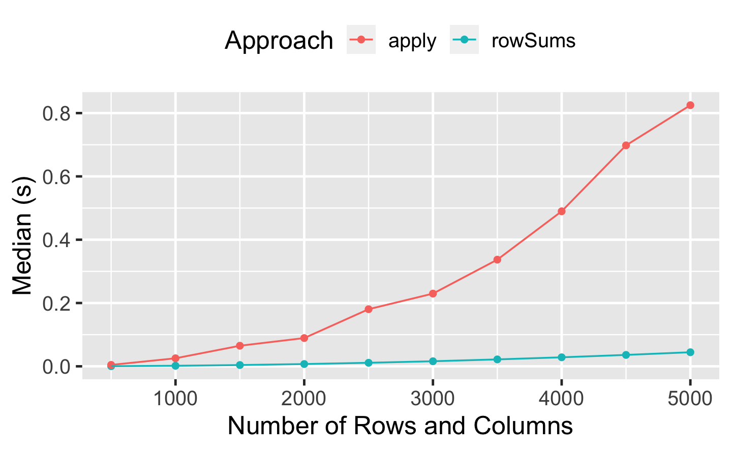

We can see that the difference in performance is negligible for small matrices but becomes more and more relevant as the size of the data increases. apply() is a very versatile tool, but it’s not “vectorised for performance” and not as optimised as rowSums().

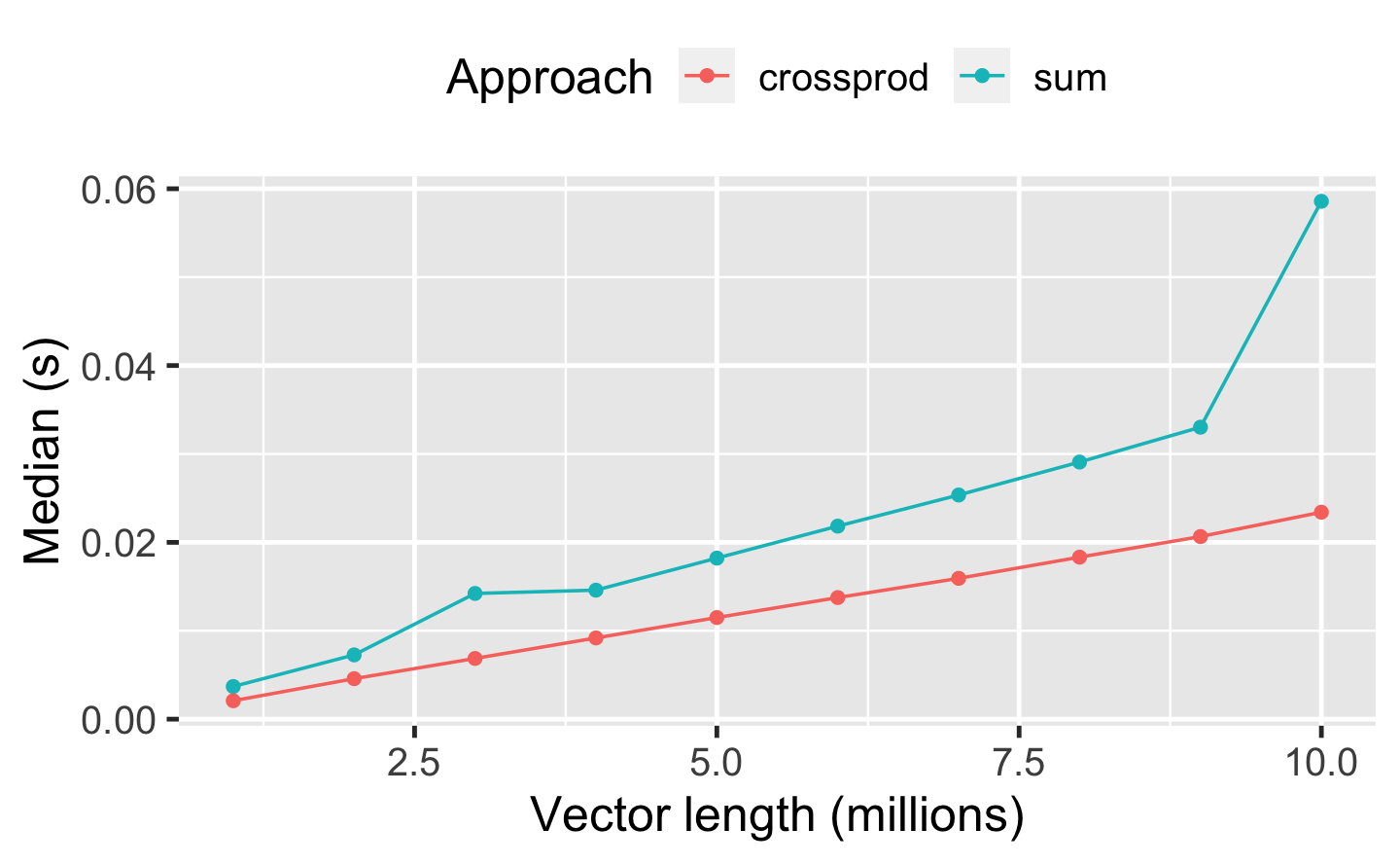
Q3: How can you use crossprod() to compute a weighted sum? How much faster is it than the naive sum(x * w)?

A: We can hand the vectors to crossprod(), which converts them to row- and column-vectors and then multiplies these. The result is the dot product, which corresponds to a weighted sum.

x <- rnorm(10)
w <- rnorm(10)
all.equal(sum(x * w), crossprod(x, w)[[1]])
#> [1] TRUE

A benchmark of both approaches for different vector lengths indicates that the crossprod() variant is almost twice as fast as sum(x * w).

weightedsum <- bench::press(
  n = 1:10,
  {
    x <- rnorm(n * 1e6)
    bench::mark(
      sum = sum(x * x),
      crossprod = crossprod(x, x)[[1]]
    )
  }
)
#> Running with:
#>        n
#>  1     1
#>  2     2
#>  3     3
#>  4     4
#>  5     5
#>  6     6
#>  7     7
#>  8     8
#>  9     9
#> 10    10

weightedsum %>%
  summary() %>%
  dplyr::mutate(Approach = as.character(expression)) %>%
  ggplot(aes(n, median, color = Approach, group = Approach)) +
  geom_point() +
  geom_line() +
  labs(x = "Vector length (millions)",
       y = "Median (s)") +
  theme(legend.position = "top")

18 Measuring performance

20 Rewriting R code in C++