8 Functionals
Prerequisites
For the functional programming part of the book, we will mainly use functions from the purrr package.14
8.1 My first functional: map()
Q1: Use as_mapper() to explore how purrr generates anonymous functions for the integer, character, and list helpers. What helper allows you to extract attributes? Read the documentation to find out.
A: map() offers multiple ways (functions, formulas, and extractor functions) to specify its function argument (.f). Initially, the various inputs have to be transformed into a valid function, which is then applied. The creation of this valid function is the job of as_mapper() and it is called every time map() is used.
Given character, numeric or list input as_mapper() will create an extractor function. Characters select by name, while numeric input selects by positions and a list allows a mix of these two approaches. This extractor interface can be very useful, when working with nested data.
The extractor function is implemented as a call to purrr::pluck(), which accepts a list of accessors (accessors “access” some part of your data object).
as_mapper(c(1, 2))  # equivalent to function(x) x[[1]][[2]]
#> function (x, ...)
#> pluck(x, 1, 2, .default = NULL)
#> <environment: 0x7fd304648470>
as_mapper(c("a", "b"))  # equivalent to function(x) x[["a"]][["b]]
#> function (x, ...)
#> pluck(x, "a", "b", .default = NULL)
#> <environment: 0x7fd30471a470>
as_mapper(list(1, "b"))  # equivalent to function(x) x[[1]][["b]]
#> function (x, ...)
#> pluck(x, 1, "b", .default = NULL)
#> <environment: 0x7fd3047952b0>
Besides mixing positions and names, it is also possible to pass along an accessor function. This is basically an anonymous function that gets information about some aspect of the input data. You are free to define your own accessor functions.
If you need to access certain attributes, the helper attr_getter(y) is already predefined and will create the appropriate accessor function for you.
# Define custom accessor function
get_class <- function(x) attr(x, "class")
pluck(mtcars, get_class)
#> [1] "data.frame"

# Use attr_getter() as a helper
pluck(mtcars, attr_getter("class"))
#> [1] "data.frame"Q2: map(1:3, ~ runif(2)) is a useful pattern for generating random numbers, but map(1:3, runif(2)) is not. Why not? Can you explain why it returns the result that it does?
A: The first pattern creates multiple random numbers, because ~ runif(2) successfully uses the formula interface. Internally map() applies as_mapper() to this formula, which converts ~ runif(2) into an anonymous function. Afterwards runif(2) is applied three times (one time during each iteration), leading to three different pairs of random numbers.
In the second pattern runif(2) is evaluated once, then the results are passed to map(). Consequently as_mapper() creates an extractor function based on the return values from runif(2) (via pluck()). This leads to three NULLs (pluck()’s .default return), because no values corresponding to the index can be found.
as_mapper(~ runif(2))
#> <lambda>
#> function (..., .x = ..1, .y = ..2, . = ..1)
#> runif(2)
#> attr(,"class")
#> [1] "rlang_lambda_function" "function"
as_mapper(runif(2))
#> function (x, ...)
#> pluck(x, 0.0807501375675201, 0.834333037259057, .default = NULL)
#> <environment: 0x7fd304ed4550>Q3: Use the appropriate map() function to:
Compute the standard deviation of every column in a numeric data frame.
Compute the standard deviation of every numeric column in a mixed data frame. (Hint: you’ll need to do it in two steps.)
Compute the number of levels for every factor in a data frame.
A: To solve this exercise we take advantage of calling the type stable variants of map(), which give us more concise output, and use map_lgl() to select the columns of the data frame (later you’ll learn about keep(), which simplifies this pattern a little).
map_dbl(mtcars, sd)
#>     mpg     cyl    disp      hp    drat      wt    qsec      vs      am    gear
#>   6.027   1.786 123.939  68.563   0.535   0.978   1.787   0.504   0.499   0.738
#>    carb
#>   1.615

penguins <- palmerpenguins::penguins

penguins_numeric <- map_lgl(penguins, is.numeric)
map_dbl(penguins[penguins_numeric], sd, na.rm = TRUE)
#>    bill_length_mm     bill_depth_mm flipper_length_mm       body_mass_g
#>             5.460             1.975            14.062           801.955
#>              year
#>             0.818

penguins_factor <- map_lgl(penguins, is.factor)
map_int(penguins[penguins_factor], ~ length(levels(.x)))
#> species  island     sex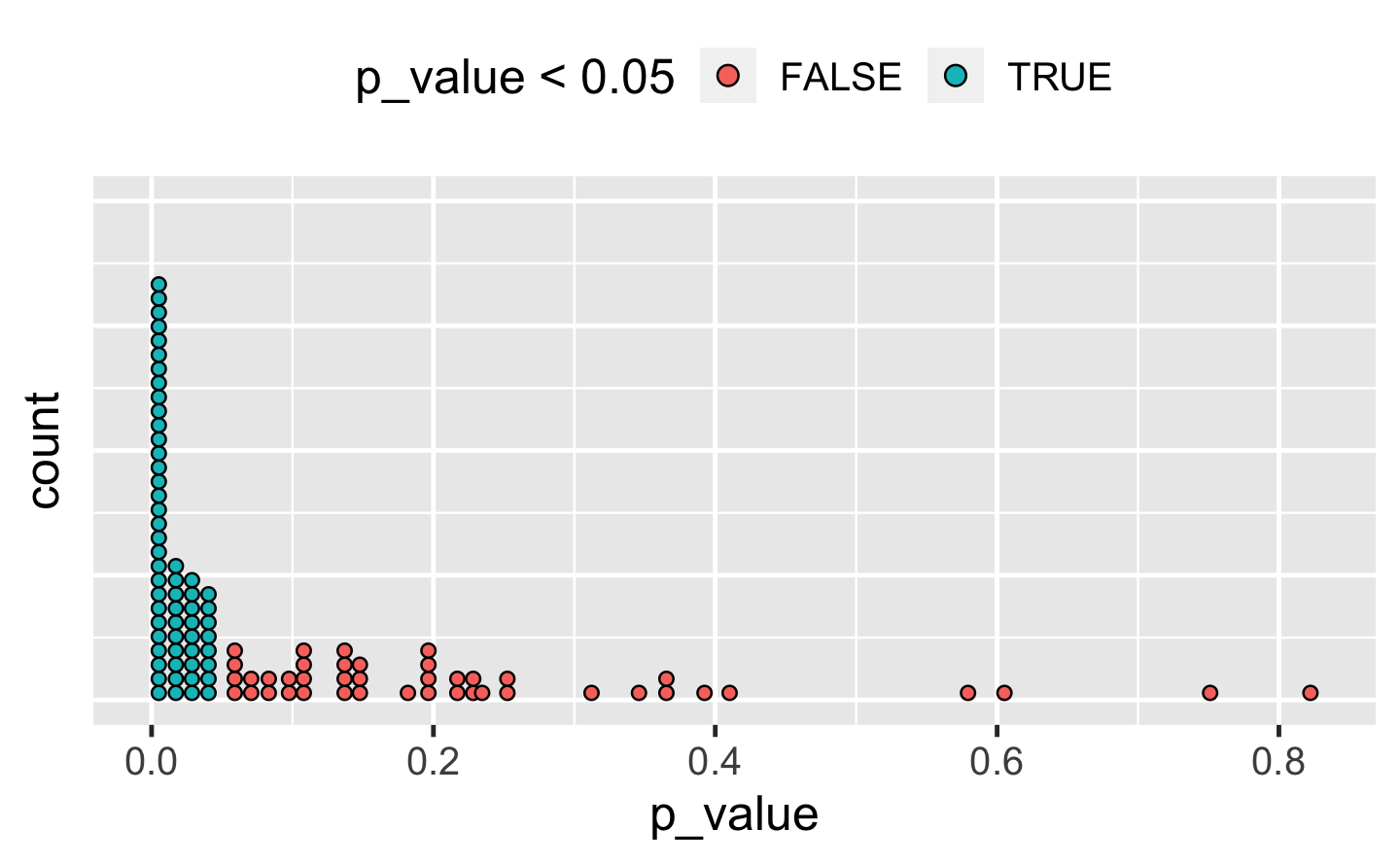
#> 3 3 2Q4: The following code simulates the performance of a t-test for non-normal data. Extract the p-value from each test, then visualise.
A: There are many ways to visualise this data. However, since there are only 100 data points, we choose a dot plot to visualise the distribution. (Unfortunately, ggplot2s geom_dotplot() doesn’t compute proper counts as it was created to visualise distribution densities instead of frequencies, so a histogram would be a suitable alternative).
library(ggplot2)

df_trials <- tibble::tibble(p_value = map_dbl(trials, "p.value"))

df_trials %>%
  ggplot(aes(x = p_value, fill = p_value < 0.05)) +
  geom_dotplot(binwidth = .01) +  # geom_histogram() as alternative
  theme(
    axis.text.y = element_blank(),
    axis.ticks.y = element_blank(),
    legend.position = "top"
  )
Q5: The following code uses a map nested inside another map to apply a function to every element of a nested list. Why does it fail, and what do you need to do to make it work?
x <- list(
  list(1, c(3, 9)),
  list(c(3, 6), 7, c(4, 7, 6))
)

triple <- function(x) x * 3
map(x, map, .f = triple)
#> Error in .f(.x[[i]], ...): unused argument (function (.x, .f, ...)
#> {
#>     .f <- as_mapper(.f, ...)
#>     .Call(map_impl, environment(), ".x", ".f", "list")
#> })A: This function call fails, because triple() is specified as the .f argument and consequently belongs to the outer map(). The unnamed argument map is treated as an argument of triple(), which causes the error.
There are a number of ways we could resolve the problem. However, there is not much to choose between them for this simple example, although it is good to know your options for more complicated cases.
# Don't name the argument
map(x, map, triple)

# Use magrittr-style anonymous function
map(x, . %>% map(triple))

# Use purrr-style anonymous function
map(x, ~ map(.x, triple))Q6: Use map() to fit linear models to the mtcars dataset using the formulas stored in this list:
A: The data (mtcars) is constant for all these models and so we iterate over the formulas provided. As the formula is the first argument of lm(), we don’t need to specify it explicitly.
models <- map(formulas, lm, data = mtcars)Q7: Fit the model mpg ~ disp to each of the bootstrap replicates of mtcars in the list below, then extract the \(R^2\) of the model fit (Hint: you can compute the \(R^2\) with summary())
bootstrap <- function(df) {
  df[sample(nrow(df), replace = TRUE), , drop = FALSE]
}

bootstraps <- map(1:10, ~ bootstrap(mtcars))A: To accomplish this task, we take advantage of the “list in, list out”-functionality of map(). This allows us to chain multiple transformations together. We start by fitting the models. We then calculate the summaries and extract the \(R^2\) values. For the last call we use map_dbl(), which provides convenient output.
8.2 Map variants
Q1: Explain the results of modify(mtcars, 1).
A: modify() is based on map(), and in this case, the extractor interface will be used. It extracts the first element of each column in mtcars. modify() always returns the same structure as its input: in this case it forces the first row to be recycled 32 times. (Internally modify() uses .x[] <- map(.x, .f, ...) for assignment.)
head(modify(mtcars, 1))
#>                   mpg cyl disp  hp drat   wt qsec vs am gear carb
#> Mazda RX4          21   6  160 110  3.9 2.62 16.5  0  1    4    4
#> Mazda RX4 Wag      21   6  160 110  3.9 2.62 16.5  0  1    4    4
#> Datsun 710         21   6  160 110  3.9 2.62 16.5  0  1    4    4
#> Hornet 4 Drive     21   6  160 110  3.9 2.62 16.5  0  1    4    4
#> Hornet Sportabout  21   6  160 110  3.9 2.62 16.5  0  1    4    4
#> Valiant 21 6 160 110 3.9 2.62 16.5 0 1 4 4Q2: Rewrite the following code to use iwalk() instead of walk2(). What are the advantages and disadvantages?
cyls <- split(mtcars, mtcars$cyl)
paths <- file.path(temp, paste0("cyl-", names(cyls), ".csv"))
walk2(cyls, paths, write.csv)A: iwalk() allows us to use a single variable, storing the output path in the names.
temp <- tempfile()
dir.create(temp)

cyls <- split(mtcars, mtcars$cyl)
names(cyls) <- file.path(temp, paste0("cyl-", names(cyls), ".csv"))
iwalk(cyls, ~ write.csv(.x, .y))
We could do this in a single pipe by taking advantage of set_names():
mtcars %>%
  split(mtcars$cyl) %>%
  set_names(~ file.path(temp, paste0("cyl-", .x, ".csv"))) %>%
iwalk(~ write.csv(.x, .y))Q3: Explain how the following code transforms a data frame using functions stored in a list.
trans <- list(
  disp = function(x) x * 0.0163871,
  am = function(x) factor(x, labels = c("auto", "manual"))
)

nm <- names(trans)
mtcars[nm] <- map2(trans, mtcars[nm], function(f, var) f(var))
Compare and contrast the map2() approach to this map() approach:
mtcars[nm] <- map(nm, ~ trans[[.x]](mtcars[[.x]]))A: In the first approach
mtcars[nm] <- map2(trans, mtcars[nm], function(f, var) f(var))the list of the 2 functions (trans) and the 2 appropriately selected data frame columns (mtcars[nm]) are supplied to map2(). map2() creates an anonymous function (f(var)) which applies the functions to the variables when map2() iterates over their (similar) indices. On the left-hand side, the respective 2 elements of mtcars are being replaced by their new transformations.
The map() variant
mtcars[nm] <- map(nm, ~ trans[[.x]](mtcars[[.x]]))does basically the same. However, it directly iterates over the names (nm) of the transformations. Therefore, the data frame columns are selected during the iteration.
Besides the iteration pattern, the approaches differ in the possibilities for appropriate argument naming in the .f argument. In the map2() approach we iterate over the elements of x and y. Therefore, it is possible to choose appropriate placeholders like f and var. This makes the anonymous function more expressive at the cost of making it longer. We think using the formula interface in this way is preferable compared to the rather cryptic mtcars[nm] <- map2(trans, mtcars[nm], ~ .x(.y)).
In the map() approach we map over the variable names. It is therefore not possible to introduce placeholders for the function and variable names. The formula syntax together with the .x pronoun is pretty compact. The object names and the brackets clearly indicate the application of transformations to specific columns of mtcars. In this case the iteration over the variable names comes in handy, as it highlights the importance of matching between trans and mtcars element names. Together with the replacement form on the left-hand side, this line is relatively easy to inspect.
To summarise, in situations where map() and map2() provide solutions for an iteration problem, several points may be considered before deciding for one or the other approach.
Q4: What does write.csv() return, i.e. what happens if you use it with map2() instead of walk2()?
A: write.csv() returns NULL. As we call the function for its side effect (creating a CSV file), walk2() would be appropriate here. Otherwise, we receive a rather uninformative list of NULLs.
8.3 Predicate functionals
Q1: Why isn’t is.na() a predicate function? What base R function is closest to being a predicate version of is.na()?
A: is.na() is not a predicate function, because it returns a logical vector the same length as the input, not a single TRUE or FALSE.
anyNA() is the closest equivalent because it always returns a single TRUE or FALSE if there are any missing values present. You could also imagine an allNA() which would return TRUE if all values were missing, but that’s considerably less useful so base R does not provide it.
Q2: simple_reduce() has a problem when x is length 0 or length 1. Describe the source of the problem and how you might go about fixing it.
simple_reduce <- function(x, f) {
  out <- x[[1]]
  for (i in seq(2, length(x))) {
    out <- f(out, x[[i]])
  }
  out
}A: The loop inside simple_reduce() always starts with the index 2, and seq() can count both up and down:
Therefore, subsetting length-0 and length-1 vectors via [[ will lead to a subscript out of bounds error. To avoid this, we allow simple_reduce() to return before the for loop is started and include a default argument for 0-length vectors.
simple_reduce <- function(x, f, default) {
  if (length(x) == 0L) return(default)
  if (length(x) == 1L) return(x[[1L]])

  out <- x[[1]]
  for (i in seq(2, length(x))) {
    out <- f(out, x[[i]])
  }
  out
}
Our new simple_reduce() now works as intended:
simple_reduce(integer(0), `+`)
#> Error in simple_reduce(integer(0), `+`): argument "default" is missing, with no default
simple_reduce(integer(0), `+`, default = 0L)
#> [1] 0
simple_reduce(1, `+`)
#> [1] 1
simple_reduce(1:3, `+`)
#> [1] 6Q3: Implement the span() function from Haskell: given a list x and a predicate function f, span(x, f) returns the location of the longest sequential run of elements where the predicate is true. (Hint: you might find rle() helpful.)
A: Our span_r() function returns the indices of the (first occurring) longest sequential run of elements where the predicate is true. If the predicate is never true, the longest run has length 0, in which case we return integer(0).
span_r <- function(x, f) {
  idx <- unname(map_lgl(x, ~ f(.x)))
  rle <- rle(idx)

  # Check if the predicate is never true
  if (!any(rle$values)) {
    return(integer(0))
  }

  # Find the length of the longest sequence of true values
  longest <- max(rle$lengths[rle$values])
  # Find the positition of the (first) longest run in rle
  longest_idx <- which(rle$values & rle$lengths == longest)[1]

  # Add up all lengths in rle before the longest run
  ind_before_longest <- sum(rle$lengths[seq_len(longest_idx - 1)])

  out_start <- ind_before_longest + 1L
  out_end <- ind_before_longest + longest
  out_start:out_end
}

# Check that it works
span_r(c(0,  0,  0,  0,  0), is.na)
#> integer(0)
span_r(c(NA, 0,  0,  0,  0), is.na)
#> [1] 1
span_r(c(NA, 0, NA, NA, NA), is.na)
#> [1] 3 4 5Q4: Implement arg_max(). It should take a function and a vector of inputs, and return the elements of the input where the function returns the highest value. For example, arg_max(-10:5, function(x) x ^ 2) should return -10. arg_max(-5:5, function(x) x ^ 2) should return c(-5, 5). Also implement the matching arg_min() function.
A: Both functions take a vector of inputs and a function as an argument. The function output is then used to subset the input accordingly.
arg_max <- function(x, f) {
  y <- map_dbl(x, f)
  x[y == max(y)]
}

arg_min <- function(x, f) {
  y <- map_dbl(x, f)
  x[y == min(y)]
}

arg_max(-10:5, function(x) x ^ 2)
#> [1] -10
arg_min(-10:5, function(x) x ^ 2)
#> [1] 0Q5: The function below scales a vector so it falls in the range [0, 1]. How would you apply it to every column of a data frame? How would you apply it to every numeric column in a data frame?
scale01 <- function(x) {
  rng <- range(x, na.rm = TRUE)
  (x - rng[1]) / (rng[2] - rng[1])
}A: To apply a function to every column of a data frame, we can use purrr::modify() (or purrr::map_dfr()), which also conveniently returns a data frame. To limit the application to numeric columns, the scoped version modify_if() can be used.
modify_if(mtcars, is.numeric, scale01)8.4 Base functionals
Q1: How does apply() arrange the output? Read the documentation and perform some experiments.
A: Basically apply() applies a function over the margins of an array. In the two-dimensional case, the margins are just the rows and columns of a matrix. Let’s make this concrete.
arr2 <- array(1:12, dim = c(3, 4))
rownames(arr2) <- paste0("row", 1:3)
colnames(arr2) <- paste0("col", 1:4)
arr2
#>      col1 col2 col3 col4
#> row1    1    4    7   10
#> row2    2    5    8   11
#> row3    3    6    9   12
When we apply the head() function over the first margin of arr2() (i.e. the rows), the results are contained in the columns of the output, transposing the array compared to the original input.
apply(arr2, 1, function(x) x[1:2])
#>      row1 row2 row3
#> col1    1    2    3
#> col2    4    5    6
And vice versa if we apply over the second margin (the columns):
apply(arr2, 2, function(x) x[1:2])
#>      col1 col2 col3 col4
#> row1    1    4    7   10
#> row2    2    5    8   11
The output of apply() is organised first by the margins being operated over, then the results of the function. This can become quite confusing for higher dimensional arrays.
Q2: What do eapply() and rapply() do? Does purrr have equivalents?
A: eapply() is a variant of lapply(), which iterates over the (named) elements of an environment. In purrr there is no equivalent for eapply() as purrr mainly provides functions that operate on vectors and functions, but not on environments.
rapply() applies a function to all elements of a list recursively. This function makes it possible to limit the application of the function to specified classes (default classes = ANY). One may also specify how elements of other classes should remain: as their identity (how = replace) or another value (default = NULL). The closest equivalent in purrr is modify_depth(), which allows you to modify elements at a specified depth in a nested list.
Q3: Challenge: read about the fixed point algorithm. Complete the exercises using R.
A: A number \(x\) is called a fixed point of a function \(f\) if it satisfies the equation \(f(x) = x\). For some functions we may find a fixed point by beginning with a starting value and applying \(f\) repeatedly. Here fixed_point() acts as a functional because it takes a function as an argument.
fixed_point <- function(f, x_init, n_max = 10000, tol = 0.0001) {
  n <- 0
  x <- x_init
  y <- f(x)

  is_fixed_point <- function(x, y) {
    abs(x - y) < tol
  }

  while (!is_fixed_point(x, y)) {
    x <- y
    y <- f(y)

    # Make sure we eventually stop
    n <- n + 1
    if (n > n_max) {
      stop("Failed to converge.", call. = FALSE)
    }
  }

  x
}


# Functions with fixed points
fixed_point(sin, x_init = 1)
#> [1] 0.0843
fixed_point(cos, x_init = 1)
#> [1] 0.739

# Functions without fixed points
add_one <- function(x) x + 1
fixed_point(add_one, x_init = 1)
#> Error: Failed to converge.