9 Function factories
Prerequisites
For most of this chapter base R15 is sufficient. Just a few exercises require the rlang,16 dplyr,17 purrr18 and ggplot219 packages.
9.1 Factory fundamentals
Q1: The definition of force() is simple:
force
#> function (x)
#> x
#> <bytecode: 0x7fe0e09464b0>
#> <environment: namespace:base>
Why is it better to force(x) instead of just x?
A: As you can see force(x) is similar to x. As mentioned in Advanced R, we prefer this explicit form, because
using this function clearly indicates that you’re forcing evaluation, not that you’ve accidentally typed
x."
Q2: Base R contains two function factories, approxfun() and ecdf(). Read their documentation and experiment to figure out what the functions do and what they return.
A: Let’s begin with approxfun() as it is used within ecdf() as well:
approxfun() takes a combination of data points (x and y values) as input and returns a stepwise linear (or constant) interpolation function. To find out what this means exactly, we first create a few random data points.
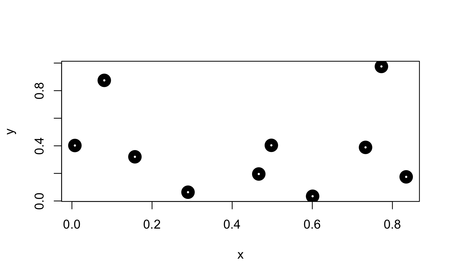
Next, we use approxfun() to construct the linear and constant interpolation functions for our x and y values.
f_lin <- approxfun(x, y)
f_con <- approxfun(x, y, method = "constant")

# Both functions exactly reproduce their input y values
identical(f_lin(x), y)
#> [1] TRUE
identical(f_con(x), y)
#> [1] TRUE
When we apply these functions to new x values, these are mapped to the lines connecting the initial y values (linear case) or to the same y value as for the next smallest initial x value (constant case).
x_new <- runif(1000)

plot(x, y, lwd = 10)
points(x_new, f_lin(x_new), col = "cornflowerblue", pch = 16)
points(x_new, f_con(x_new), col = "firebrick", pch = 16)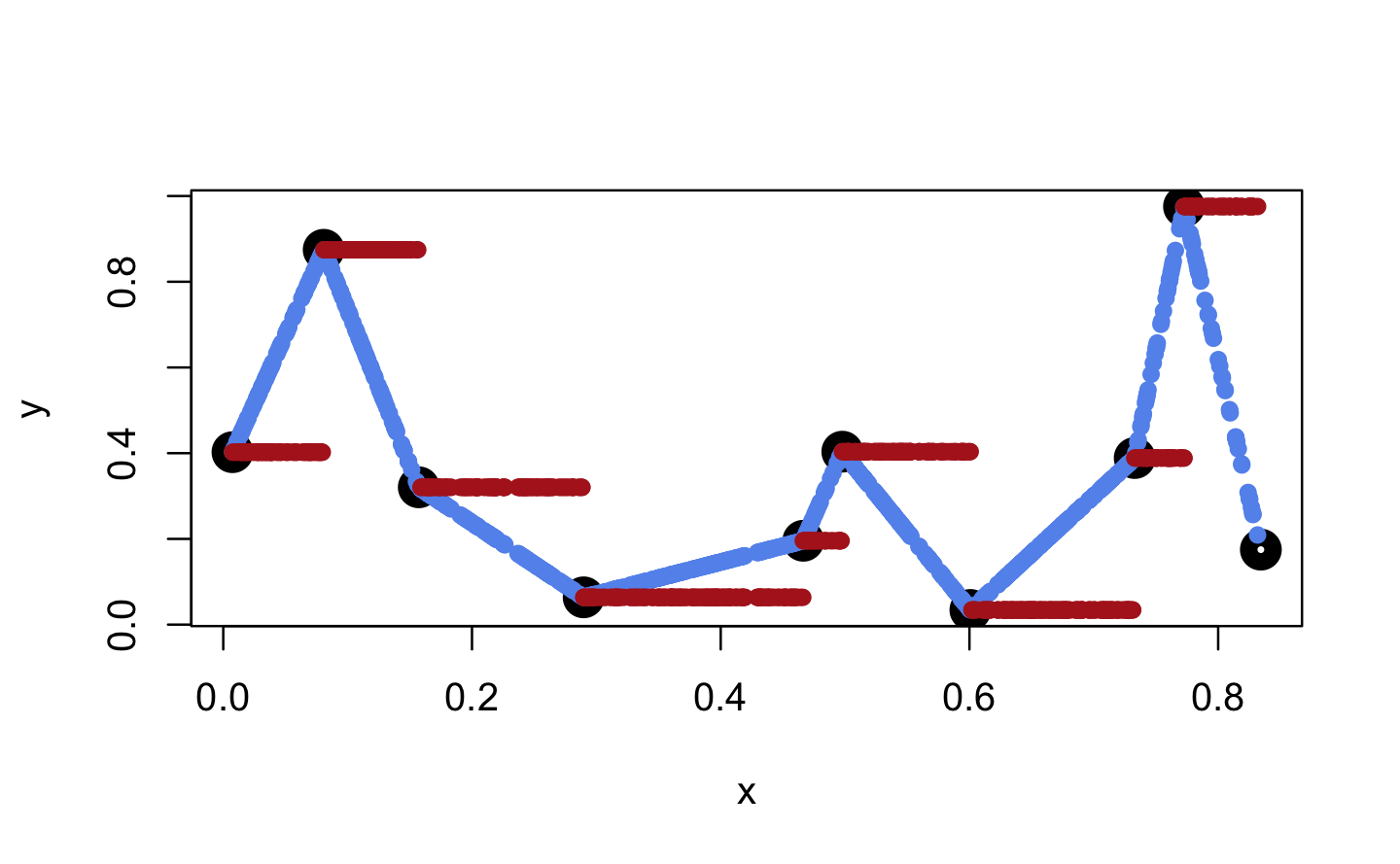
However, both functions are only defined within range(x).
f_lin(range(x))
#> [1] 0.402 0.175
f_con(range(x))
#> [1] 0.402 0.175

(eps <- .Machine$double.neg.eps)
#> [1] 1.11e-16

f_lin(c(min(x) - eps, max(x) + eps))
#> [1] NA NA
f_con(c(min(x) - eps, max(x) + eps))
#> [1] NA NA
To change this behaviour, one can set rule = 2. This leads to the result that for values outside of range(x) the boundary values of the function are returned.
f_lin <- approxfun(x, y, rule = 2)
f_con <- approxfun(x, y, method = "constant", rule = 2)

f_lin(c(-Inf, Inf))
#> [1] 0.402 0.175
f_con(c(-Inf, Inf))
#> [1] 0.402 0.175
Another option is to customise the return values as individual constants for each side via yleft and/or yright.
f_lin <- approxfun(x, y, yleft = 5)
f_con <- approxfun(x, y, method = "constant", yleft = 5, yright = -5)

f_lin(c(-Inf, Inf))
#> [1]  5 NA
f_con(c(-Inf, Inf))
#> [1]  5 -5
Further, approxfun() provides the option to shift the y values for method = "constant" between their left and right values. According to the documentation this indicates a compromise between left- and right-continuous steps.
f_con <- approxfun(x, y, method = "constant", f = .5)

plot(x, y, lwd = 10)
points(x_new, f_con(x_new), pch = 16)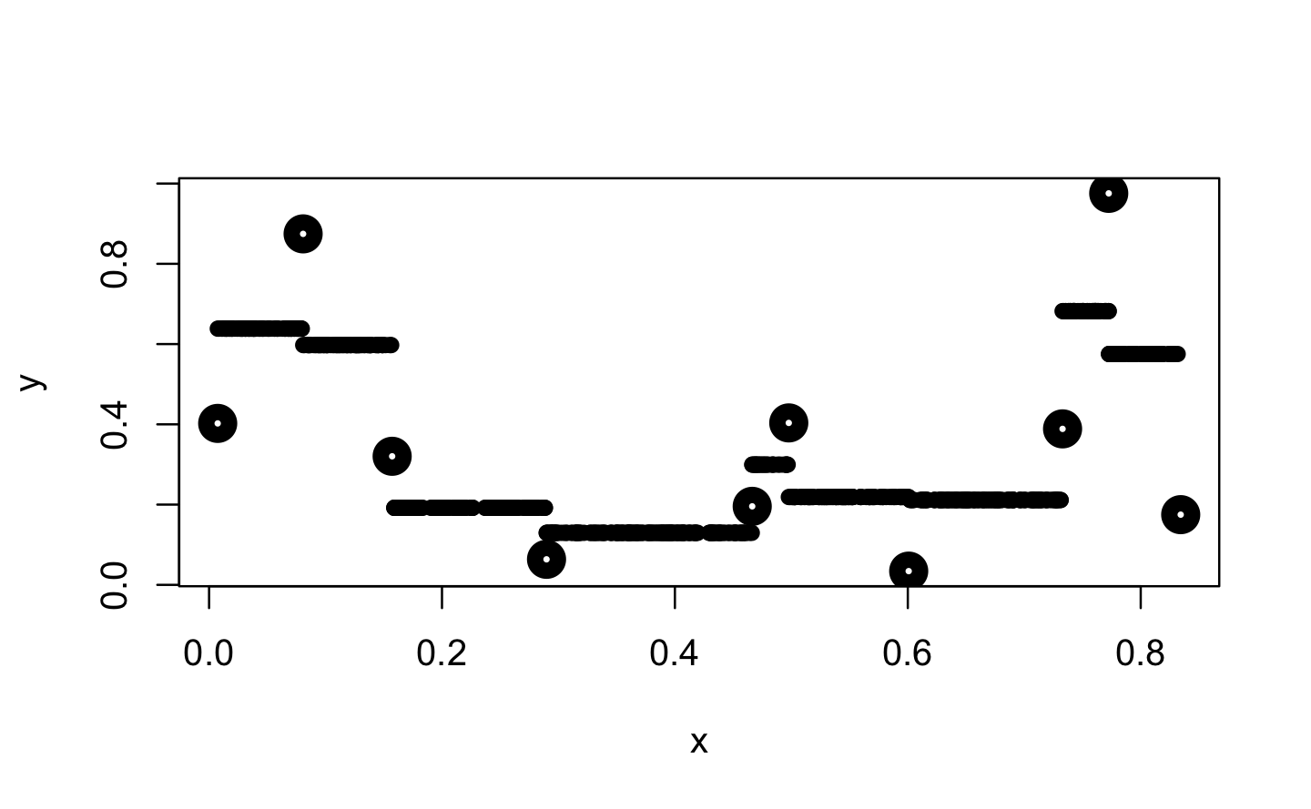
Finally, the ties argument allows to aggregate y values if multiple ones were provided for the same x value. For example, in the following line we use mean() to aggregate these y values before they are used for the interpolation approxfun(x = c(1,1,2), y = 1:3, ties = mean).
Next, we focus on ecdf(). “ecdf” is an acronym for empirical cumulative distribution function. For a numeric vector of density values, ecdf() initially creates the (x, y) pairs for the nodes of the density function and then passes these pairs to approxfun(), which gets called with specifically adapted settings (approxfun(vals, cumsum(tabulate(match(x, vals)))/n, method = "constant", yleft = 0, yright = 1, f = 0, ties = "ordered")).
x <- runif(10)
f_ecdf <- ecdf(x)
class(f_ecdf)
#> [1] "ecdf"     "stepfun"  "function"

plot(x, f_ecdf(x), lwd = 10, ylim = 0:1)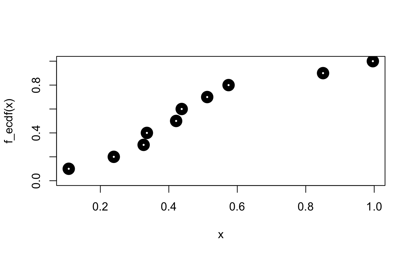
New values are then mapped on the y value of the next smallest x value from within the initial input.
x_new <- runif(1000)

plot(x, f_ecdf(x), lwd = 10, ylim = 0:1)
points(x_new, f_ecdf(x_new), ylim = 0:1)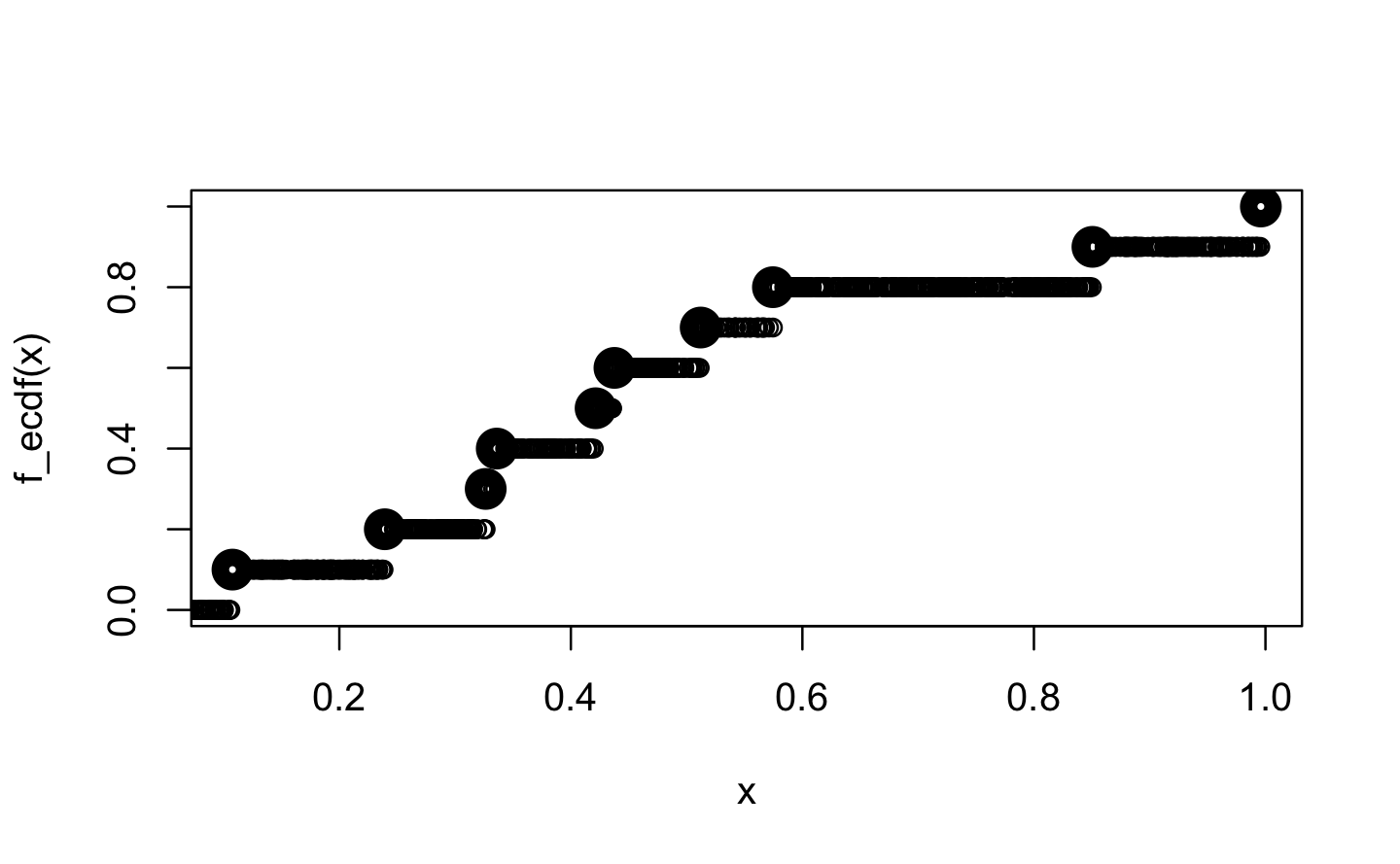
Q3: Create a function pick() that takes an index, i, as an argument and returns a function with an argument x that subsets x with i.
pick(1)(x)
# should be equivalent to
x[[1]]

lapply(mtcars, pick(5))
# should be equivalent to
lapply(mtcars, function(x) x[[5]])A: In this exercise pick(i) acts as a function factory, which returns the required subsetting function.
pick <- function(i) {
  force(i)

  function(x) x[[i]]
}

x <- 1:3
identical(x[[1]], pick(1)(x))
#> [1] TRUE
identical(
  lapply(mtcars, function(x) x[[5]]),
  lapply(mtcars, pick(5))
)
#> [1] TRUEQ4: Create a function that creates functions that compute the ithcentral moment of a numeric vector. You can test it by running the following code:
m1 <- moment(1)
m2 <- moment(2)

x <- runif(100)
stopifnot(all.equal(m1(x), 0))
stopifnot(all.equal(m2(x), var(x) * 99 / 100))A: The first moment is closely related to the mean and describes the average deviation from the mean, which is 0 (within numerical margin of error). The second moment describes the variance of the input data. If we want to compare it to var(), we need to undo Bessel’s correction by multiplying with \(\frac{N-1}{N}\).
moment <- function(i) {
  force(i)

  function(x) sum((x - mean(x)) ^ i) / length(x)
}

m1 <- moment(1)
m2 <- moment(2)

x <- runif(100)
all.equal(m1(x), 0)  # removed stopifnot() for clarity
#> [1] TRUE
all.equal(m2(x), var(x) * 99 / 100)
#> [1] TRUEQ5: What happens if you don’t use a closure? Make predictions, then verify with the code below.
i <- 0
new_counter2 <- function() {
  i <<- i + 1
  i
}A: Without the captured and encapsulated environment of a closure the counts will be stored in the global environment. Here they can be overwritten or deleted as well as interfere with other counters.
new_counter2()
#> [1] 1
i
#> [1] 1
new_counter2()
#> [1] 2
i
#> [1] 2

i <- 0
new_counter2()
#> [1] 1
i
#> [1] 1Q6: What happens if you use <- instead of <<-? Make predictions, then verify with the code below.
new_counter3 <- function() {
  i <- 0
  function() {
    i <- i + 1
    i
  }
}A: Without the super assignment <<-, the counter will always return 1. The counter always starts in a new execution environment within the same enclosing environment, which contains an unchanged value for i (in this case it remains 0).
new_counter_3 <- new_counter3()

new_counter_3()
#> [1] 1
new_counter_3()
#> [1] 1
9.2 Graphical factories
Q1: Compare and contrast ggplot2::label_bquote() with scales::number_format().
A: Both functions will help you in styling your output, e.g. in your plots and they do this by returning the desired formatting function to you.
ggplot2::label_bquote() takes relatively straightforward plotmath expressions and uses them for faceting labels in ggplot2. Because this function is used in ggplot2 it needs to return a function of class = "labeller".
scales::number_format() initially force()s the computation of all parameters. It’s essentially a parametrised wrapper around scales::number() and will help you format numbers appropriately. It will return a simple function.
9.3 Statistical factories
Q1: In boot_model(), why don’t I need to force the evaluation of df or model?
A: boot_model() ultimately returns a function, and whenever you return a function you need to make sure all the inputs are explicitly evaluated. Here that happens automatically because we use df and formula in lm() before returning the function.
boot_model <- function(df, formula) {
  mod <- lm(formula, data = df)
  fitted <- unname(fitted(mod))
  resid <- unname(resid(mod))
  rm(mod)

  function() {
    fitted + sample(resid)
  }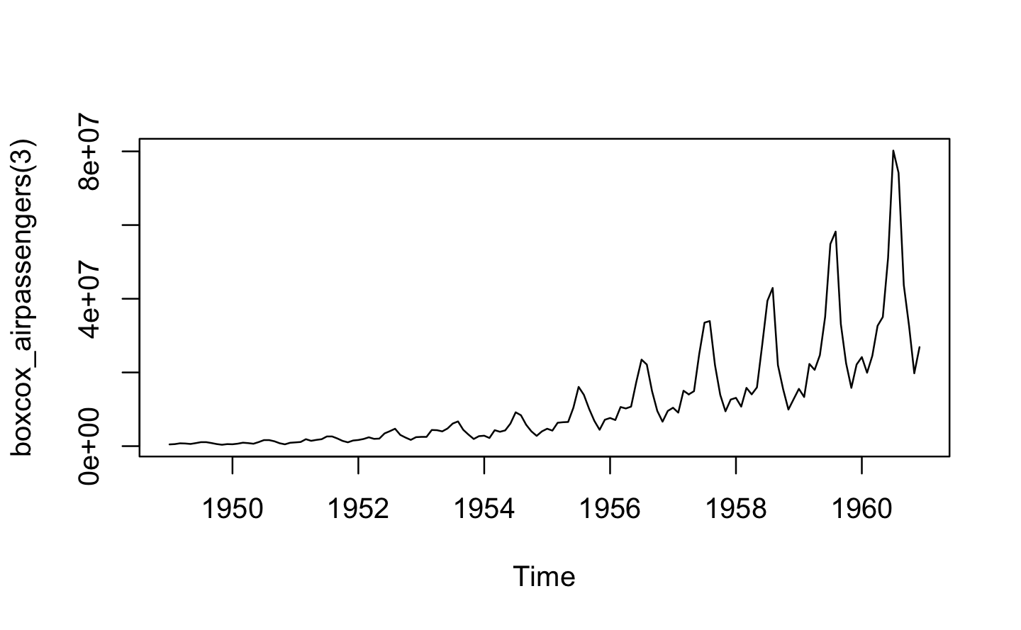
} Q2: Why might you formulate the Box-Cox transformation like this?
boxcox3 <- function(x) {
function(lambda) {
if (lambda == 0) {
log(x)
} else {
(x ^ lambda - 1) / lambda
}
}
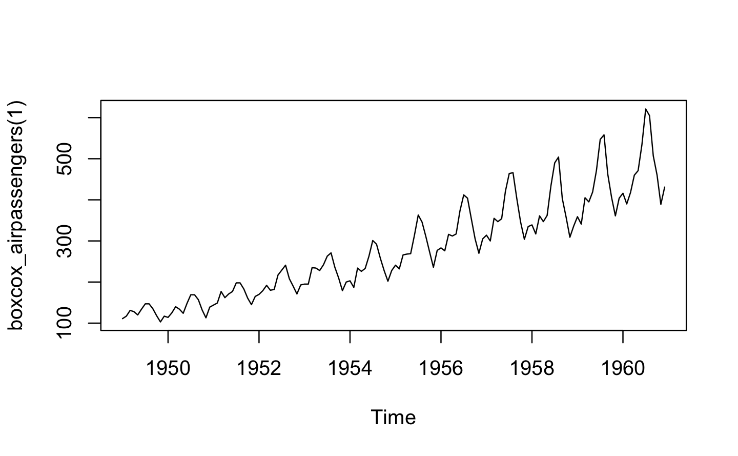
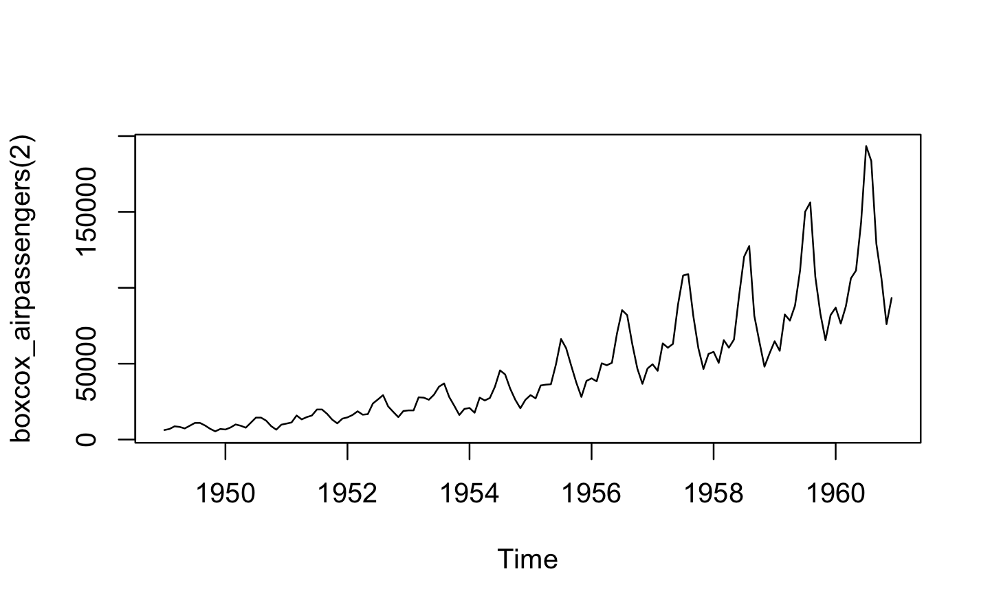
}A: boxcox3() returns a function where x is fixed (though it is not forced, so it may be manipulated later). This allows us to apply and test different transformations for different inputs and give them a descriptive name.
boxcox_airpassengers <- boxcox3(AirPassengers)

plot(boxcox_airpassengers(0))
plot(boxcox_airpassengers(1))
plot(boxcox_airpassengers(2))
plot(boxcox_airpassengers(3))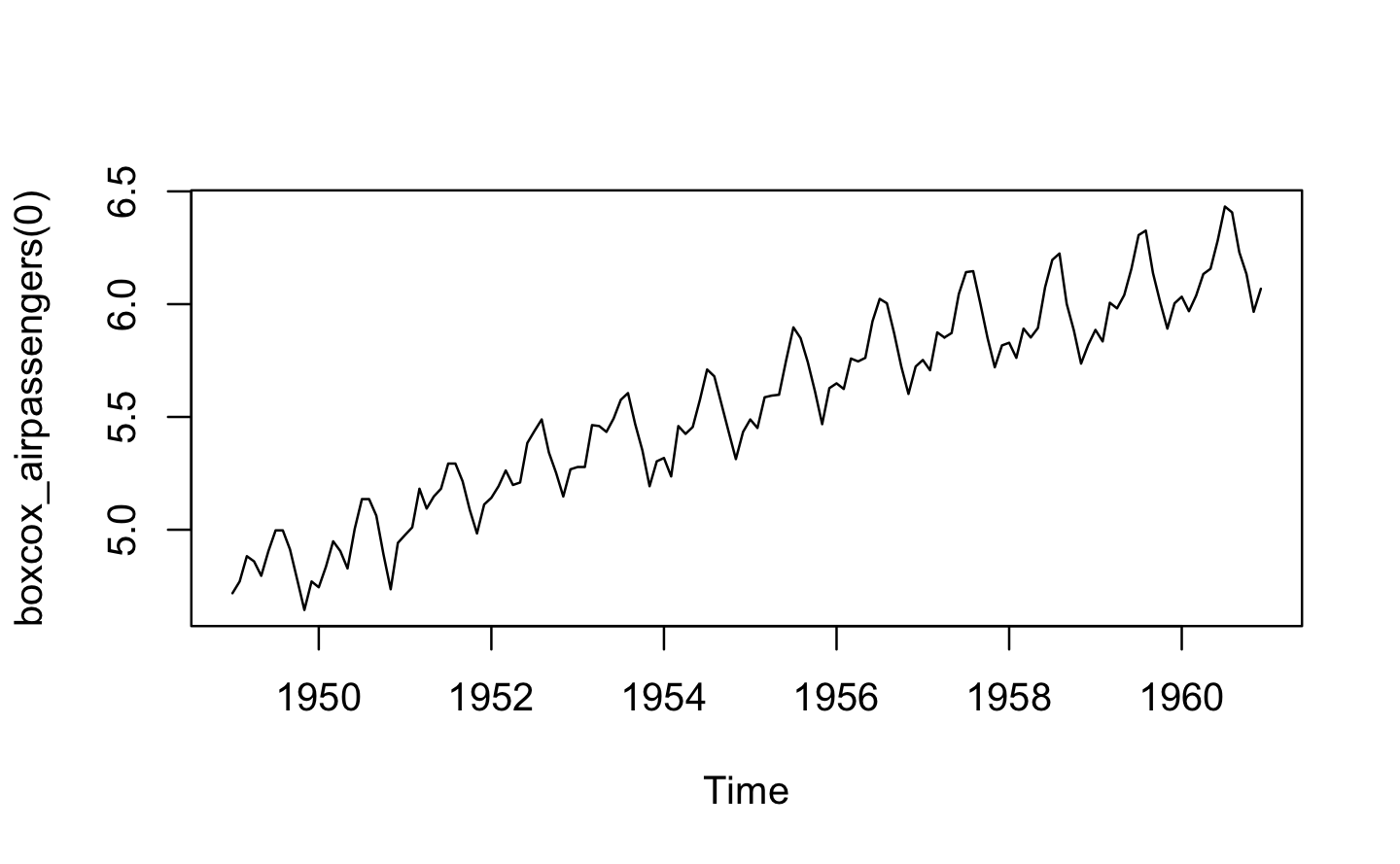
Q3: Why don’t you need to worry that boot_permute() stores a copy of the data inside the function that it generates?
A: boot_permute() is defined in Advanced R as:
boot_permute <- function(df, var) {
  n <- nrow(df)
  force(var)

  function() {
    col <- df[[var]]
    col[sample(n, replace = TRUE)]
  }
}
We don’t need to worry that it stores a copy of the data, because it actually doesn’t store one; it’s just a name that points to the same underlying object in memory.
boot_mtcars1 <- boot_permute(mtcars, "mpg")

lobstr::obj_size(mtcars)
#> 7,208 B
lobstr::obj_size(boot_mtcars1)
#> 20,248 B
lobstr::obj_sizes(mtcars, boot_mtcars1)
#> *  7,208 B
#> * 13,040 BQ4: How much time does ll_poisson2() save compared to ll_poisson1()? Use bench::mark() to see how much faster the optimisation occurs. How does changing the length of x change the results?
A: Let us recall the definitions of ll_poisson1(), ll_poisson2() and the test data x1:
ll_poisson1 <- function(x) {
  n <- length(x)

  function(lambda) {
    log(lambda) * sum(x) - n * lambda - sum(lfactorial(x))
  }
}

ll_poisson2 <- function(x) {
  n <- length(x)
  sum_x <- sum(x)
  c <- sum(lfactorial(x))

  function(lambda) {
    log(lambda) * sum_x - n * lambda - c
  }
}

x1 <- c(41, 30, 31, 38, 29, 24, 30, 29, 31, 38)
A benchmark on x1 reveals a performance improvement of factor 2 for ll_poisson2() over ll_poisson1():
bench::mark(
  llp1 = optimise(ll_poisson1(x1), c(0, 100), maximum = TRUE),
  llp2 = optimise(ll_poisson2(x1), c(0, 100), maximum = TRUE)
)
#> # A tibble: 2 x 6
#>   expression      min   median `itr/sec` mem_alloc `gc/sec`
#>   <bch:expr> <bch:tm> <bch:tm>     <dbl> <bch:byt>    <dbl>
#> 1 llp1         49.3µs   54.7µs    17761.    12.8KB     22.1
#> 2 llp2         26.8µs   30.1µs    31795.        0B     22.3
As the redundant calculations within ll_poisson1() become more expensive with growing length of x1, we expect even further relative performance improvements for ll_poisson2(). The following benchmark reveals a relative performance improvement of factor 20 for ll_poisson2() when x1 is of length 100,000:
bench_poisson <- function(x_length) {
  x <- rpois(x_length, 100L)

  bench::mark(
    llp1 = optimise(ll_poisson1(x), c(0, 100), maximum = TRUE),
    llp2 = optimise(ll_poisson2(x), c(0, 100), maximum = TRUE),
    time_unit = "ms"
  )
}

performances <- map_dfr(10^(1:5), bench_poisson)

df_perf <- tibble(
  x_length = rep(10^(1:5), each = 2),
  method   = rep(attr(performances$expression, "description"), 5),
  median   = performances$median
)

ggplot(df_perf, aes(x_length, median, col = method)) +
  geom_point(size = 2) +
  geom_line(linetype = 2) +
  scale_x_log10() +
  labs(
    x = "Length of x",
    y = "Execution Time (ms)",
    color = "Method"
  ) +
  theme(legend.position = "top")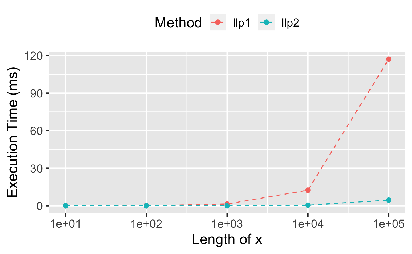
9.4 Function factories + functionals
Q1: Which of the following commands is equivalent to with(x, f(z))?
-
x$f(x$z). -
f(x$z). -
x$f(z). -
f(z). - It depends.
A: (e) “It depends” is the correct answer. Usually with() is used with a data frame, so you’d usually expect (b), but if x is a list, it could be any of the options.
f <- mean
z <- 1
x <- list(f = mean, z = 1)

identical(with(x, f(z)), x$f(x$z))
#> [1] TRUE
identical(with(x, f(z)), f(x$z))
#> [1] TRUE
identical(with(x, f(z)), x$f(z))
#> [1] TRUE
identical(with(x, f(z)), f(z))
#> [1] TRUEQ2: Compare and contrast the effects of env_bind() vs. attach() for the following code.
funs <- list(
  mean = function(x) mean(x, na.rm = TRUE),
  sum = function(x) sum(x, na.rm = TRUE)
)

attach(funs)
#> The following objects are masked from package:base:
#>
#>     mean, sum
mean <- function(x) stop("Hi!")
detach(funs)

env_bind(globalenv(), !!!funs)
mean <- function(x) stop("Hi!")
env_unbind(globalenv(), names(funs))A: attach() adds funs to the search path. Therefore, the provided functions are found before their respective versions from the {base} package. Further, they cannot get accidentally overwritten by similar named functions in the global environment. One annoying downside of using attach() is the possibility to attach the same object multiple times, making it necessary to call detach() equally often.
attach(funs)
#> The following objects are masked from package:base:
#>
#>     mean, sum
attach(funs)
#> The following objects are masked from funs (pos = 3):
#>
#>     mean, sum
#>
#> The following objects are masked from package:base:
#>
#>     mean, sum

head(search())
#> [1] ".GlobalEnv"      "funs"            "funs"            "package:ggplot2"
#> [5] "package:purrr"   "package:dplyr"
detach(funs)
detach(funs)
In contrast rlang::env_bind() just adds the functions in fun to the global environment. No further side effects are introduced, and the functions are overwritten when similarly named functions are defined.